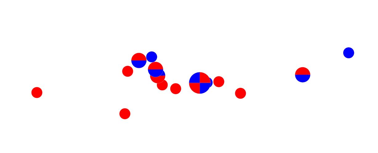
Plot foliations and lineations as colored dots at the outcrop localities on SVG map with color representing dip- or plunge-direction
Bas den Brok - mapping course

Understanding of python, SVG and some understanding of Dutch required.


We have a txt file with structure data e.g. foliations (azimuth and dip) and coordinates (SVG coordinates) and want to spatially plot them in SVG format and give them a color according to which side they are dipping towards, e.g. plotting a red dot when dipping towards the east and a blue dot when dipping towards the west. When more than one measurement was made at one locality i.e. one outcrop then the dot should have a surface twice as big and color as in a piechart. The program can deal with up to twelve measurements per locality (dots twelve times as big and 12 pieces are colored).

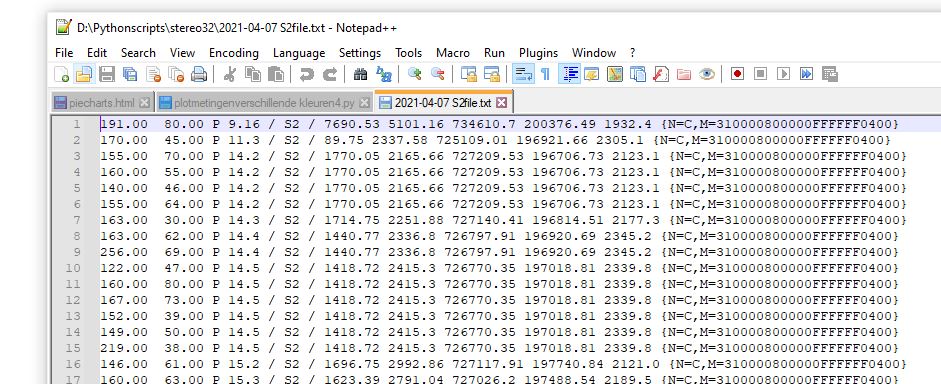
The input file is a txt file in stereo32 format of S2 measurements such as the one here below showing azimuth, dip, outcrop number, SVG- and Swissgrid CH1903 coordinates an elevation as well as layout info for stereo32 between curly brackets:

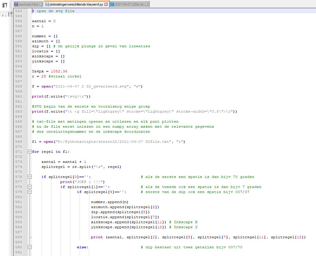
Here is the entire Python file: plotmetingenverschillende kleuren4.py (not for use! Only to help you write your own program.) The programs start with reading the relevant values from the txt file into a numpy array:

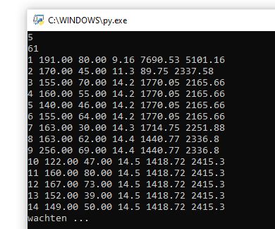
The screen output first shows the relevant values azimuth, dip, outcrop number and SVG-coordinates stored into the nupy array. The numbers 5 and 61 corrspond to the number of characters written to the first two lines of the SVG file:

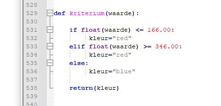
In this specific case we wanted to color the foliations with a dip in the range 346 degrees NNW clockwise to 166 degrees SSE red (i.e. more or less the east dipping ones) and the the other ones (the west dipping ones) blue as defined in lines 529-538. You can easily change criteria there. NOte: azimuth input values between 0 and 360.

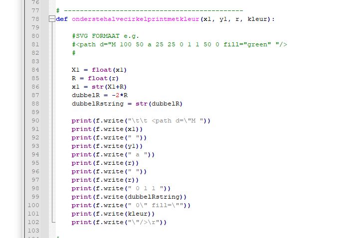
Plotting one measurement on one locality as a circle is easy. Plotting more then one is a bit complicated. Plotting for example one of two measurements on one licality required plotting two half spheres. For example, the code of the lower half sphere was defined as below:

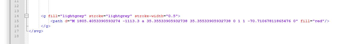
Resulting SVG-code looks like:

and in Inkscape like:

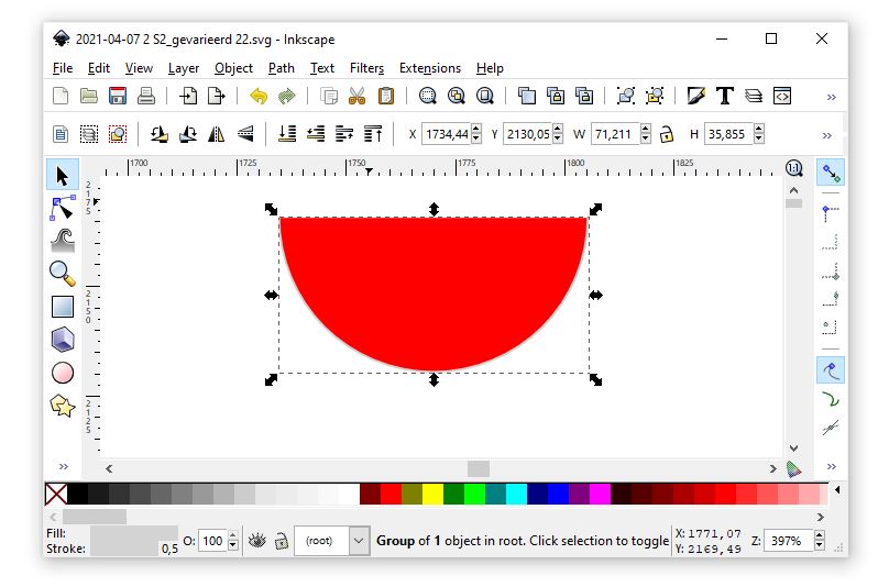
in Inkscape the final result may like here below. Of course the size of the dots can easily be adjusted in the Python program in line 556 by changing radius r set to 25 in the present example:

an example of six measurements on one locality:

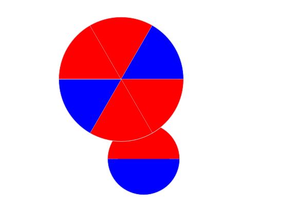
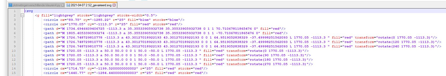
the resulting SVG-file looks like here below. The circle-tags in lines 3, 4, 14 and 15 are for single measurements on a locality, the path-tags of lines 5 and 6 correspond to two neasurments on only locality. (The above half sphere is the one of line 6.) The paths online 7, 8 amd 9 are for three measurments on one locality and paths 10, 11, 12 and 13 for four measurements i.e. four quarters making up one dot.: